3D骨骼系统的几种用例的配置方案

我前面已经总结了两篇文章来研究3D骨骼系统的底层实现原理运作机制。本文来探索一下3D骨骼系统的实际应用问题。这里提出几种实际的应用情况与3D骨骼系统的配置方案。

对所有的实际3D骨骼应用情况,我们分两种情况,第一,骨骼与被控对象位置重和的情况。第二,骨骼与被控对象分离的情况。第一种情况对应着three.js系统中skinnedMesh.bindMode === 'attached', 第二种情况对应skinnedMesh.bindMode === 'detached'。看下图示例:

其中,红色的线条代表骨骼,黑色的代表SkinnedMesh。在attached模式下,被控对象通过bindMatrix移动到骨骼所在位置,然后骨骼的运动直接控制几何顶点的运动。在实际应用中为了实现这种方案,我们有两种方案。

  1. 把受控对象的位置直接调整到骨骼所在的位置,然后只需要运行skinnedMesh.bind(skeleton)绑定起来即可。或者先把受控对象初始位置摆好,然后再配置好骨骼的位置来匹配这些受控对象。
  2. 先把骨骼摆好,然后每一个受控对象通过配置一个bindMatrix,将受控对象移动到骨骼的相应位置。此时,需要skinnedMesh.bind(skeleton, bindMatrix)

在有的情况,被控对象与骨骼在位置上是不直接影响的。我们希望骨骼的运动在跨越一段空间后再同步的去影响受控对象。此时就需要detached模式了。如上图右边所示,如果我们希望骨骼绕自己转30度,受控对象也绕自己的某个点转30度。假设,受控对象的该点到骨骼的转移矩阵为M,那么我们就需要这样来配置骨骼系统了:

skinnedMesh.bind(skeleton, M)
skinnedMesh.bindMode = 'detached'

需要注意的是,这里的M是不考虑skinnedMesh的matrixWorld在内的转移矩阵。detached模式下,matrixWorld是自由的,能够完全决定skinnedMesh所在的位置。

detach的绑定模式下,可以轻松的实现一个骨架控制多个处于不同位置的受控对象做同步运动。

深度解析3D骨骼系统中骨骼运动对几何体顶点运动的影响

前文中,我已经总结了3D骨骼系统的底层运作原理。现在我将更进一步解析骨骼的运动对几何体顶点运动的影响。three.js实现骨骼控制的代码中引用了一个bindMatrix变量,这个bindMatrix在很多应用的场景下,我们都不用管它,因为在默认的情况下,bindMatrix等于初始化时与之对应SkinnedMesh的matrixWrold。但其实bindMatrix对骨骼运动与几何顶点运动的影响是比较大的。我们可以看下一段glsl代码:

export default /* glsl */`     
#ifdef USE_SKINNING
                     
  vec4 skinVertex = bindMatrix * vec4( transformed, 1.0 );
                            
  vec4 skinned = vec4( 0.0 );
  skinned += boneMatX * skinVertex * skinWeight.x;
  skinned += boneMatY * skinVertex * skinWeight.y;
  skinned += boneMatZ * skinVertex * skinWeight.z;
  skinned += boneMatW * skinVertex * skinWeight.w;
                                                        
  transformed = ( bindMatrixInverse * skinned ).xyz;
                                                                               
#endif
`;

在对几何顶点应用骨骼转移矩阵的时候,这里首先把顶点通过bindMatrix矩阵来转移。要解释这样做对结果的影响,我需要借助以下图来表达:

其中蓝色是骨骼bone,红点是没有通过bindMatrix转移的点,绿点是通过bindMatrix转移后的点。我们假设bone, 做了一个相对自己所在的点的旋转运动,并转过了alpha个角度。那么,按照图示,此运动对红点所的影响向量为a,对绿点影响向量为b。注意了,这里判断bone对几何点的影响方式可以看成这样:1.首先把几何点看成与bone的本地坐标系的相对位置是固定不变的。2. 当bone坐标系发生移动后,几何点做相同的运动。这里的相同是指相对全局坐标系的相同运动。例如bone绕自己转了alpha个角度,那么相对于全局坐标系,bone是做了绕bone所在坐标点做了alpha角度的转动。很显然,a和b是不一样的,bindMatrix直接影响了骨骼运动对几何顶点的影响值。

3D骨骼系统中,对几何顶点的变化顺序如下:

  1. 将所有顶点按照bindMatrix的矩阵数据做变化。
  2. 接着,顶点数据按照每个骨骼在全局坐标系下相对初始化是的变化矩阵做相应的权值变化。
  3. 随后,顶点按照bindMatrixInverse数据做变化。
  4. 最后顶点按照其自身SkinnedMesh的matrixWorld做变化

这里,需要特别注意的是,bindMatrixInverse不一定就是bindMatrix的逆。它由SkinnedMesh的bindMode来控制。bindMode为'attached'的时候,bindMatrixInverse是matrixWorld的逆,bindMode为'detached'的时候,bindMatrixInverse才是bindMatrix的逆。所以根据bindMode的不同值,上述的顺序可以简化表达如下:

bindMode等于'attached'时:

  1. 将所有顶点按照bindMatrix的矩阵数据做变化。
  2. 接着,顶点数据按照每个骨骼在全局坐标系下相对初始化是的变化矩阵做相应的权值变化。

这里的3,4步骤可以被省略掉,因为bindMatrixInverse一定是matrixWorld的逆,它们互相抵消。

bindMode等于'detached'时:

  1. 所有顶点做一个受bone权值影响的变化,相应bone对顶点的影响向量由顶点经过bindMatrix位置变化后,相对bone的位置所决定。
  2. 顶点按照其自身SkinnedMesh的matrixWorld做变化

这里,因为bindMatrixInverse与bindMatrix互逆,bindMatrixInverse能抵消掉顶点按照bindMatrix的移动,但时保留了顶点按照骨骼权值的运动影响。

3D骨骼模型的底层原理

3D骨骼模型在计算机图形学的某些应用上有很重要的地位,尤其是需要用到动画或者变形的3D模型。我们平时能接触到的各种图形引擎都实现了对3D骨骼模型的支持。本文以three.js为例,介绍一下3D骨骼模型实现的底层原理。

为了实现骨骼3D模型的系统,three.js提供了3个对象来达到目的 ———SkinnedMesh, Bone, Skeleton。对于整个骨骼体系而言,这3个对象并不是平等的关系,他们是从属关系。其中Skeleton在整个3D骨骼体系中起到一个总体的架构作用,无论是SkinnedMesh还是Bone都可以看作是Skeleton的组成部分。在three.js中,他们以不同的形式来实现与Skeleton的关系。

Skeleton定义了一个模型的所有关节结构。每一个skeleton的关节可以理解为一个点,这个点拥有记录空间位姿的所有数据,此外这个关节还拥有一个parent和children的拓扑结点的结构。大体来说,在three.js中,这个关节点基本上等价于一个Object3D。而这样一个关节点的载体就是Bone。因此,我们可以将Skeleton理解为Bone的容器,它管理着这些Bone的结构并且记录它们的初始位姿。

这里,很有意思的一点。Skeleton是通过记录那些Bone的初始矩阵的逆来记录它们的初始位置。为何如此?假设每个Bone的初始矩阵为m0,m0的逆为m0-1,Bone在经过一系列变化之后的矩阵为m1,而这一系列的变化矩阵为mt,则: mt*m0 = m1,那么mt = m1 * m0-1。如此我们调整完每一个Bone时,都能轻松的通过m0-1和矩阵的当前的数据m1来求得Bone的转移矩阵。

那么,拿到了转移矩阵后要怎么办?这就要提到SkinnedMesh了。不同于一般的Mesh,最重要的一点,SkinnedMesh的geometry中除了position, normal 等这些常见属性外,它还有skinIndex和skinWeight这两个属性。

每一个SkinnedMesh都可以与Skeleton绑定,而SkinnedMesh中geometry的skinIndex是一个4元数组,其中每一个元素是指向4个bone的指引。然后skinWeight也是一个4元数组,不过这里面每一个元素是指每一个相对应bone的影响权重。

这样skinIndex和skinWeight就建立了Skeleton中bone对geometry中position的影响。请看下面一段来自three.js中glsl的代码片段:

export default /* glsl */`     
#ifdef USE_SKINNING
                     
  vec4 skinVertex = bindMatrix * vec4( transformed, 1.0 );
                            
  vec4 skinned = vec4( 0.0 );
  skinned += boneMatX * skinVertex * skinWeight.x;
  skinned += boneMatY * skinVertex * skinWeight.y;
  skinned += boneMatZ * skinVertex * skinWeight.z;
  skinned += boneMatW * skinVertex * skinWeight.w;
                                                        
  transformed = ( bindMatrixInverse * skinned ).xyz;
                                                                               
#endif
`;


export default /* glsl */`     
#ifdef USE_SKINNING
                     
  mat4 boneMatX = getBoneMatrix( skinIndex.x );            
  mat4 boneMatY = getBoneMatrix( skinIndex.y );
  mat4 boneMatZ = getBoneMatrix( skinIndex.z );
  mat4 boneMatW = getBoneMatrix( skinIndex.w );    
                                                   
#endif                                             
`;     

代码中,transformed最后用来计算gl_Position的值。我们可以清晰的看到skinIndex和skinWeight是如何影响transformed的值。getBoneMatrix函数是通过指引来读取与SkinnedMesh所绑定的Skeleton中Bone的相对转移矩阵。

SkinnedMesh是最后被显卡渲染的对象,整个骨骼体系,本质上可以这么理解:3D骨骼体系建立Bone对SkinnedMesh中几何顶点的权值影响关系。而由于这层关系是通过显卡应用建立起来的,因此Bone的位姿值在变化后,实现的几何变形会非常的快速。

如果,放到three.js这里,这句话可以更精确点说成:threejs的3D骨骼体系建立了最多支持4个骨骼位姿数据对SkinnedMesh中几何顶点的权值影响关系。

通过上面的解释,我们也能理解,这个关系是通过Skeleton建立起来的。

MatCap材质简介

MatCap材质,有时候也叫做发光球材质。它是自2007年zbrush软件应用此材质开始,在全球范围内流行起来的一种材质。这种材质的特点是能够用一张纹理图来表现材质在某个具体环境下向不同方向给出的反射效果。看下图所示:

右侧图片中的球,定义了从正面看,一个球上不同的点的颜色各有不同。它定义了与摄像头视角成不同方向夹角的法线所应该表现的颜色。图片的左侧应用的就是右侧球为纹理的matcap材质。可以看得到,凡是该3D对象中法线方向与右侧球上左上方法线方向一致的点都是高亮的颜色。

MatCap材质通过一张纹理来表现环境中的灯光效果,但于此同时,在实时渲染中,它却没有用到光线渲染的运算。既节省了渲染资源,又表达了渲染效果。

此材质的缺点也很明显,那就是不能适应变化的复杂环境。它所表现的,永远是发光球所处的环境。

mesh建模的核心技术——曲面细分算法简析

   不同于实体建模的表面网格(mesh)建模被广泛应用在艺术品,游戏角色等3D模型的构建之中。而在mesh建模发展的历史过程中,最惹人瞩目的技术恐怕非“曲面细分”(subdivision)算法莫属。而曲面细分算法的各种方案中又以Catmull-Clark方案最为应用广泛。致力于研究曲面细分算法的研发和优化的工程师们在业界满载着荣誉。例如在曲面细分算法上做出突出贡献的Jos Stam就曾经获得过SGI公司颁发的"计算机图形奖",并两次获得“奥斯卡科技成果奖”(这也侧面说明曲面细分算法对电影事业的重大影响)。
      下面将简要的解析Catmull-Clark算法。
      后文来自http://www.rorydriscoll.com/2008/08/01/catmull-clark-subdivision-the-basics/

A LITTLE BACKGROUND FIRST

How exactly does a 3D application decide how to subdivide a control mesh? Well, there are a few different subdivision schemes out there, but the most widely used is Catmull-Clark subdivision. Since the original paper by Ed Catmull and Jim Clark, there have been a number of improvements to the original scheme, in particular dealing with crease and boundary edges. This means that although an application might say that it uses Catmull-Clark subdivision, you’ll probably see slightly different results, particularly in regard to edge weights and boundaries.

RULES OF SUBDIVISION

The original rules for how to subdivide a control mesh are actually fairly simple. The paper describes the mathematics behind the rules for meshes with quads only, and then goes on to generalize this without proof for meshes with arbitrary polygons. I’m going to go through a very simple example here to show what happens when a mesh gets subdivided. I’m going to be concentrating solely on non-boundary sections of the mesh for simplicity. Also, the example uses a 2D mesh, but again this is only for simplicity, and the principles expand to 3D without change.

There are four basic steps to subdividing a mesh of control-points:

1. Add a new point to each face, called the face-point.
2. Add a new point to each edge, called the edge-point.
3. Move the control-point to another position, called the vertex-point.
4. Connect the new points.

Easy, right? The only question left to answer is, what are the rules for adding and moving these points? Well, like I wrote earlier, this really depends on who implemented it, but I’m going to show the original Catmull-Clark rules using screenshots from Modo. This doesn’t mean that these are the rules that Modo applies, but it should be fairly close.

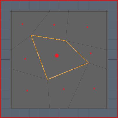
Here’s the example mesh I’m going to be using:


No prizes for guessing which face we’re going to be looking at. I’ve made it a little bit skewed because that makes things more interesting. If you’re wondering about the double edges around the boundary, I’m going to be writing about those at a later date, so be patient! For now I need them to make the boundary hold shape, but they can be safely ignored for the purposes of this article.

STEP ONE

Firstly, we need to insert a face point, but where? Well this is easy, it just needs to go at the average position of all the control points for the face:


I’ve drawn red dots approximately where each new face-point will go. The big dot is obviously the face-point for the highlighted face. The location for each dot is simply the sum of all the positions of the control-points in that face, divided by the number of control-points.

STEP TWO

Now we need to add edge-points. Because we’re not dealing with weighted, crease or boundary edges, this is also fairly simple. For each edge, we take the average of the two control points on either side of the edge, and the face-points of the touching faces.

Here’s an example for one edge-point, in blue, where the control points affecting its position are pink, and face-points are red. Note that the edge points don’t necessarily lie on the original edge!


For the highlighted face only, I’ve drawn all the roughly where each new edge-point will go in blue:

STEP THREE

This step is a little bit more complicated, but very interesting. We’re going to see how we place the vertex-points from the original control points, and why they get placed there. This time, we use a weighted average to determine where the vertex-point will be placed. A weighted average is just a normal average, except you allow some values to have greater influence on the final result than others.

Before I begin with the details of this step, I need to define a term that you may have heard used in regards to subdivision surfaces – valence. The valence of a point is simply the number of edges that connect to that point. In the example mesh, you can see that all of the control points have a valence of 4.
Alright, I’m going to dive into some math here, but I’m also going to explain what the math actually means in real terms, so don’t be put off!

The new vertex-point is placed at:

(Q/n) + (2R/n) + (S(n-3)/n)

where n is the valence, Q is the average of the surrounding face points, R is the average of all surround edge midpoints, and S is the control point.

When you break this down, it’s actually fairly simple. Looking at our example, our control-points have a valence of 4, which means n = 4. Applying this to the formula, we now get:

(Q/4) + (R/2) + (S/4)

Much simpler! What does this mean though? Well, it says that a quarter of the weighting for the vertex-point comes from the average of surrounding face-points, half of it comes from the surrounding edge midpoints, and the last quarter comes from the original control-point.

If we look at the top left control point in the highlighted face, Q is the average of the surrounding face-points, the red dots:


R is the average of the surrounding edge midpoints, the yellow dots. Note that the yellow dots represent the middle of the edge (just the average of the two end points) which is a little bit different from the edge-points we inserted above because they don’t factor in the nearby face-points.

S is just the original control-point, the pink dot:

Below is my rough approximation of where all these averages come out, using the same color scheme as before. So the yellow dot is the average of all the yellow dots above, and the red dot is the average of all the red dots above.


Now all we do is take the weighted average of these points. So remember that the red dot accounts for a quarter, the yellow dot accounts for half, and the pink dot accounts for the final quarter. So the final resting place for the vertex-point should be somewhere near the yellow dot, slightly toward the pink dot, roughly where the pink dot is below:


So now I hope you can see why the control point is going to get pulled down and to the right. All the surrounding points just get averaged together and weighted to pull the vertex around. This means that if a control-point is next to a huge face, and three small faces, the huge face is going to pull that vertex towards it much more that the small faces do.

One other thing you can see from this is that if the mesh is split into regular faces, then the control point won’t move at all because the average of all the points will be the same as the original control point. The pull from each face-point and edge midpoint gets canceled out by a matching point on the other side:

STEP FOUR

The final step is just to connect all the points. Confusingly, Modo has two ways to subdivide a mesh which actually return slightly different results. I don’t know why this is, or how the subdivision schemes differ, but they are close enough for all intents and purposes to call the same. For clarity, I’m using a screenshot from Modo where I have subdivided using the SDS subdivide command. For the highlighted face only, I’ve drawn the new face-point in red, the new edge-points in blue, and the moved vertex-points in pink:


Below is an overlay of the original control mesh for reference. As expected, you can see that the top left control-point gets pulled to the right. The same process is applied to all faces, resulting in four times as many quads as we had previously.

ONE MORE THING

If you look at the formula for moving the control-point to its new location, you can see that not only are the immediate neighbor points used, so are the all the rest of the points in the adjoining faces. How much any single one of these surrounding points affects the control-point isn’t very clear from the original formula. This information is actually really easy to find out just by substituting in the surrounding points into the original formula.

I’m making the assumption from hereon out that all of the surrounding faces are quads to make things easier on myself. Also, I’m not going to write down each step of the expansion here since it got pretty big, but at the end, I got the following weights:

Control-point weight = (4n-7) / 4n
Edge-neighbor weight = 3 / 2n^2
Face-neighbor weight = 1 / 4n^2

I’m using the term edge-neighbor to denote a neighboring point sharing the same edge as the control point, and face-neighbor as a neighbor that only shares the same face as the control-point. In the picture below, the edge-neighbors are cyan, and the face neighbors are yellow. Note that for quads, you have exactly n edge-neighbors, and n face-neighbors.

Applying this formula to various different valences, you get the following weights for a single point of the given type:

Valence
Control
Edge Neighbor
Face Neighbor
35/123/181/36
49/163/321/64
513/203/501/100
Infinity100

What does this mean? If we look at a the valence-4 row, you can see that if you move a face-neighbor, that’s going to affect the position of the vertex-point by 1/64th of however much you move it. So if you move it 64 cm on the x-axis, then the resulting vertex-point will move 1 cm in the same direction. I tested this scenario out in Modo, and it seems to match up very closely.

Clearly, the edge-neighbors are weighted more heavily than the face-neighbors, and the control-point itself always the most influence on the final vertex-point location. Remember though, each point represents a different thing (control-point, edge-neighbor, face-neighbor, nothing) depending on which particular face is getting subdivided!

It is interesting to note what happens as the valence gets larger and larger. The control-point influence tends towards 1, while all the neighboring points tend to zero. The reverse is also true, where at valence-4, the control-point weight is about 0.56, at valence-3 it is only 0.41 which means it is getting pulled around by its neighbors a lot more.

mipmap在3d图形渲染的用法

一个图片mipmap,指的是一系列的图形队列。队列中的没个图形都是对于原始图形不同分辨率的复制。但时这个分别率的取值是有讲究的,它必须是2的指数次。以下是一组mipmap分辨率的示例:

原始图像 265*512, mipmap中分辨率: [128*256, 64*128, 32*64, 16*32, 8*16, 4*8,2*4,1*2]

可见mipmap中的分辨率在宽和高两个方向上都是原始图像中2的指数上递减的队列。

mipmap的在3d渲染中主要带来两个优点: 提升渲染速度和减少锯齿。同一个3D对象的纹理在渲染时可以根据其与摄像头的距离调整纹理的分辨率。这可以很有效的减少渲染的时间。另外,由于远距离对象的纹理分辨率降低,这也减少了锯齿的发生。

在渲染引擎中各种类型纹理的解释

在很多时候,我们所提到的纹理,似乎都是指一张图片。这张图片按照一个指定的映射方法,把像素映射到3D对象的表面上去。但实际上纹理能做的事情远超这种简单的应用。

我想其实可以给纹理一个更加广义的定义:纹理是用来控制物体表面的物理性质,从而增强应用对3D模型表面的表达能力。而这些物理性质,大多表现在对光的反应情况。有时候,它反应的是光线照过来之后,散射出来的光应该是什么颜色,有时候它反应的是光线照过来之后反射光的方向,或者是同一束光照过来之后,有多少强度被按反射角的方向反射回去,有多少被散射开来。等等,这些一系列描述物体表面上某个点在收到光线后的反应数据。描述不同的物理原理的数据被称为各种不同类型的原理。

下面我们将分别解释这些纹理的作用

颜色纹理 (colormap)

颜色纹理是最常见的纹理,它反应的是物体表面的颜色。一般不加任何说明时,我们通常指的纹理就是这个纹理。

向量纹理 和凹凸纹理 (normal map and bump map)

在不同的软件不同的应用中有时候会区别对待向量纹理和凹凸纹理,有时候一个应用中的这两个纹理是同一个意思。但无论是那种情况,向量纹理和凹凸纹理都是用来控制材质表面对光线的反射方向的。向量纹理数据可以指定物体表面的法向量,从而进一步实现对光线的反射方向做出控制。这样,贴上向量纹理的光滑表面就能给人肉眼感觉出凹凸不平的感觉。

在有一些应用或渲染引擎中,如three.js,它在一些材质中除了normal纹理还额外的定义了bump纹理。在这里,bump是简化版的normal纹理。normal纹理的每个点要通过3维的数据来控制物体表面的法向量,而bump只需要一个数以及一个总体上的系数来表示表面的凹凸程度就可以了。bump纹理通过描述凹凸程度来表达物体表面的法向量。

位移纹理 (displacement map)

有时候仅仅通过上文所提到的向量纹理或凹凸纹理来达到物体表面情况的表达是不够的。位移纹理能实际的改变物体表面的几何凹凸形状,因此位移纹理可以在需要表示凹凸程度比较大而且几何建模又不太方便的时候使用。

反射纹理 (specular map or reflection map)

反射纹理用来表达物体表面对光线的反射情况

光泽度(粗糙度)纹理 (gloss or roughness)

光泽度和粗糙度在定义纹理时是一对反义词,因此它们内部是可以互相转化的。与反射纹理对比,粗糙度和光泽度本质上是从另外一套数学模型下来描述物体表面对光线的反射情况。

金属度纹理 (metalness)

金属对光照的反射情况与非金属是不一样的。这里其实与光泽纹理,反射纹理目的是一样,就是想要控制物体表面对光照的反射情况。只不过金属度纹理采用了不一样的数学模型来表达数据对光线的反射影响。如果,有一个3D对象同时存在多个对光线反射的纹理,例如:同时存在反射纹理,金属度纹理,则物体最终对光线的反射情况是这些纹理效用的叠加。

环境遮挡纹理 (ao map)

环境遮挡纹理是用来描述物体表面被光线的遮挡程度,它能反应物体表面上某个点在当前环境下总体上的明暗程度。这个纹理配合其他纹理使用时能表达物体表面上的阴影效果。

光线纹理(light map)

光线纹理也主要是反应物体表面的阴影情况,只是有时候与ao map不同的是,光线纹理用来描述表达物体在一个具体场景下,物体表面光线的阴影情况。而ao map反应的是当前场景下受环境光影响的阴影情况。对边ao map和light map的烘培图,我们应该就能体会到它们之间的差异。

环境纹理 (env map)

环境纹理在应用时能反应一个物体表面所对的环境的颜色。

上图中,球面贴的就是它当前所处环境的纹理。它本质上是颜色纹理,只是对环境贴图的映射到物体表面的映射方法由所不同。如果环境贴图是一个天空盒子,6张图。那么环境纹理在应用时需要建立环境贴图的6个图映射到物体的各各相应位置处。

threejs阴影的渲染机制

理解threejs阴影的渲染机制,对控制阴影的产生性能可以有很大的帮助。本文将对threejs阴影的形成做个简要概述。

threejs中阴影的形成分两步,首先threejs会渲染出针对castShadow和receiveShadow的设定,对每个receiveShadow的面生成一个阴影纹理,然后再把这个纹理给贴在该面上。给每个面贴纹理需要一定计算量,给每次面更新纹理也需要计算量。这两个计算量的存在,有时候能很大幅度的影响一个场景在低端机器上的渲染性能。

因此,threejs的WebglRenderer特别的推出了一个属性renderer.shadowMap.autoUpdate。我们可以给这个属性配置为false从而关闭每次移动摄像头或者添加无关紧要的对象等操作而导致的shadowMap的更新,从而避免上文中提到的第一步的运算量。

正如,下文对阴影提到的问题一样:

If your scene is static, only update the shadow map when something changes, rather than every frame

Use a CameraHelper to visualize the shadow camera’s viewing frustum

Remember that point light shadows are more expensive than other shadow types since they must render six times (once in each direction), compared with a single time for DirectionalLight and SpotLight shadows

While we’re on the topic of PointLight shadows, note that the CameraHelper only visualizes one out of six of the shadow directions when used to visualize point light shadows. It’s still useful, but you’ll need to use your imagination for the other 5 directions

threejs的渲染顺序

threejs的渲染顺序有时候会对场景成像效果产生严重的影响。这一切的源头都来自于opengl的一种深度优化的工作原理。opengl会对需要渲染的对象做深度探测,也就是所谓的depthTest。当它发现需要渲染的部分被距离摄像头更近的对象遮挡住的时候,就会不再对其进行渲染。这种机制,本能的减少了gpu的工作量,优化了渲染性能。为了更好的利用这个特性,threejs会对需要渲染的非透明对象进行一次按距离摄像头从近到远的排序(近远的判断是根据object的boundingSphere属性)。如此,距离摄像头越近的对象就会越被先渲染,距离摄像头越远的对象会被后渲染,这样就能更快发现后面的对象的哪些个点会被遮住,从而避免对该点的渲染计算。然而,对于透明对象(transparent === true),threejs会按照距离摄像头从远到近的顺序来进行渲染,这样就能避免距离摄像头远的透明物体被因为depthTest的机制而取消渲染。

还有一点,就是透明的物体都是渲染在非透明的物体之后。这样做的原因无它,也就是想要避免因depthTest机制的存在而导致放在透明物体后面的非透明物体没有被渲染。

那么问题来了,如果两个对象距离摄像头的距离一样呢?这确实就是很多图像显示的罪恶之源。threejs就会不知道先渲染哪个,这会导致偶发性的z-fighting。在一些个别或者任何的摄像头位置,一些像素点显示的颜色不断的在两个对象间切换,甚至是有些对象出现可视与不可视之间不断的跳变。像这种情况,通常的解决方法,有三种。第一,关闭某个对象的depthTest, 让它能无视渲染顺序,从而确保其会被渲染,而不会因为depthTest的存在而变得不可见。第二,关闭某个对象的depthWrite,让该对象的的数据不会被写入gpu的深度缓存中,从而,其他对象在做depthTest的时候,就不会发现它挡在了前面。第三,人为的设定对象的渲染顺序。每个threejs对象都会有一个renderOrder属性,我们可以人为地配置对象A的renderOrder小于B的renderOrder,这样,就算A按照前文的机制因该渲染在B之后,但由于renderOrder的原因,能而改变此规则,让A渲染在B之前。

后处理中bloom与outline的实现原理

bloom与outline是后处理中最常用的两个效果,这里对它们的实现原理做个基本的介绍。

bloom

bloom即是所谓的绽放效果,它能让3D对象产生“亮闪闪”的特效。让人感觉该3D对象能够发光,而且光线能够延伸到3D对象以外的空间。这种特效得益于三个后处理步骤。第一,通过一种机制将发光部分的计准图片从3D渲染得到的图片中选择出来(抠图)。这种方法可以有很多,例如,可以设定一个发光度阈值,对2维图片做个高通滤波,把一张图片中亮度高的像素点选择出来,以仅仅含有这些高像素点的图片为计准。也可以一开始先设定一些3D对象,先对整个场景有选择的对3D对象做可视性的设定,先对这些希望能让其发光的对象先做渲染,然后以这张图片为发光特效生成的基准。有了基准图片后,接着可以对此图片做多次的高斯模糊处理,让基准图片上的像素像四周延伸。最后,再把这张有选择性的,向四周延伸图片与正常场景的图片做一个混色合成。大功告成,最后得到了一张看起来图片中有部分在发光而且还影响到了其周围的物体。

outline

理解了bloom的机制,再来理解outline的工作机制就轻松一些了。其实它们的步骤差不多:第一,做选择。将需要描绘outline的部件选择出来,对这些部件单独做深度渲染到一张图片。第二,对这个做了深度渲染图片做边界的渲染,这可能包括边界的识别,边界的高斯模糊处理。第三,渲染一张正常的图片后,再把前一张图片与这张正常图片做混色合成。这就是outline的工作机制。